Adjusting historical prices for stock splits and dividends keeps a change in share structure or a cash distribution from masquerading as a trading gain or loss. Without those adjustments, a stock split can look like a collapse, and a dividend payment can distort the return earned by a shareholder.
The right adjustment depends on the question. Reconstructing an actual trade requires prices available in that session. Comparing investment performance requires accounting for distributions. Building indicators requires consistent units across the entire calculation window. One price column should not do all three jobs.
This guide covers the adjustment calculations, worked examples, and checks needed before using corporate action data in research or a trading system. For broader issues such as missing observations and inconsistent timestamps, start with historical market data quality and cleaning.
Raw Prices, Split Adjusted Prices, and Total Returns
Separate three concepts before changing any data:
| Data series | What it represents | Typical use |
|---|---|---|
| Raw prices | Historical prices in the share units traded at the time | Execution simulation and historical price filters |
| Split adjusted prices | Historical prices converted to a common share basis | Price comparisons and indicators across splits |
| Dividend adjusted or total return series | A series incorporating distributions under a stated calculation method | Investment performance and return comparisons |
Total return includes price changes and dividend income, but the reinvestment convention matters. A gross return calculation uses dividends before withholding deductions; a net return calculation applies the methodology’s withholding assumptions. These distinctions appear in the S&P Dow Jones Indices total return methodology. Neither measure should be mistaken for an individual investor’s return after every tax, fee, and trading cost.
For a simple holding period without a split, the gross return is:
Return = (ending price + dividend per share) ÷ starting price − 1
If a stock starts at $100, ends at $102, and distributes $2 per share, the return is 4%, not the 2% shown by the price change alone. Across several periods, compound the period returns rather than adding them.
How to Adjust Historical Prices for Stock Splits
A split changes the number of shares represented by a holding. To compare prices across the event, convert earlier observations into the later share units.
Define the split ratio as new shares divided by old shares. A 2-for-1 split has a ratio of 2. A 1-for-10 reverse split has a ratio of 0.1.
For backward adjustment to the post-split basis:
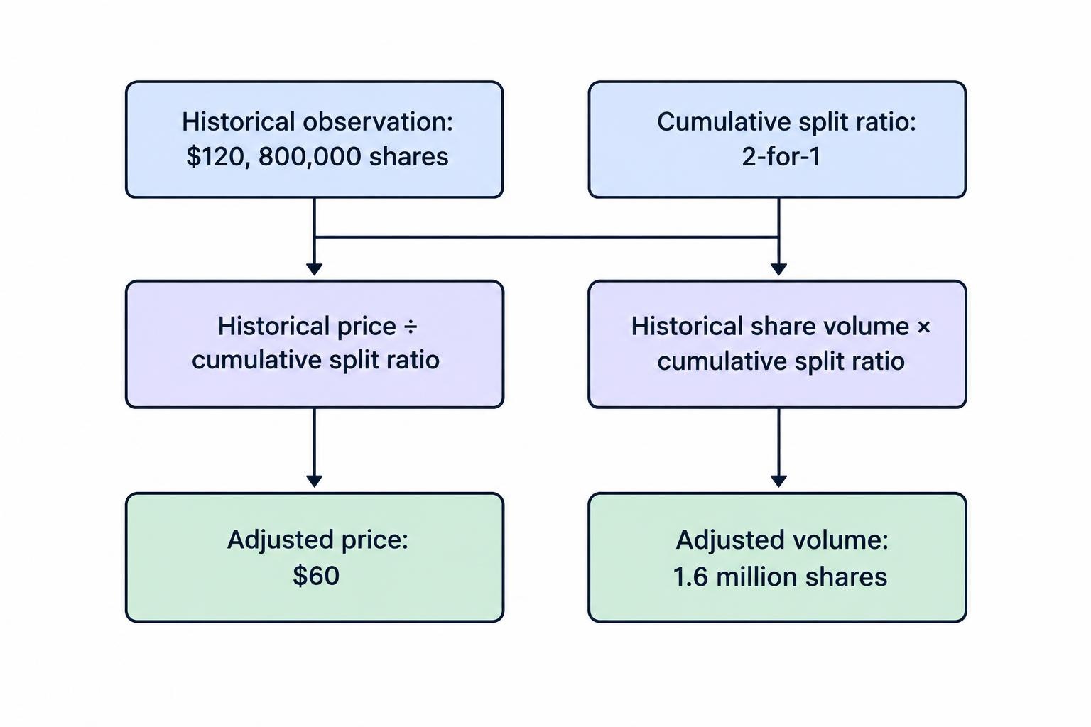
Adjusted historical price = raw historical price ÷ split ratio
Adjusted historical share volume = raw historical share volume × split ratio
Prices and share volume move in opposite directions because the unit being counted changes. This treatment is demonstrated in Massive’s split adjustment example for prices and volume.
A 2-for-1 Split Example
Consider a hypothetical stock closing at $120 before a 2-for-1 split and $61 in the first post-split session. Comparing the raw closes produces an apparent loss of about 49.17%.
Divide the earlier close by two. The comparable prices become $60 and $61, producing a gain of approximately 1.67%.
The holding tells the same story. An investor with 100 shares worth $12,000 before the event has 200 shares worth $12,200 afterward. The split itself does not create the $200 gain; the move from the equivalent $60 price to $61 does.
If the earlier session recorded 800,000 shares traded, its volume becomes 1.6 million shares on the post-split basis. This is a unit conversion, not evidence of extra trading.
Reverse Splits and Multiple Events
For a 1-for-10 reverse split, divide earlier prices by 0.1, which multiplies them by ten. Multiply historical share volume by 0.1. A pre-event price of $2 therefore becomes $20 on the new basis.
For multiple splits, multiply the ratios of all events between the observation and the chosen adjustment date. A 2-for-1 split followed by a 3-for-1 split produces a cumulative ratio of six. A $180 observation before both events becomes $30.
Apply only the events that occur after each observation. A price recorded between those two splits needs the later factor of three, not the full factor of six.
How Dividend Adjustments Work
A cash dividend needs different treatment because it distributes value without changing the shareholder’s share count. The calculation must distinguish a price return from a return that includes the distribution.
One backward adjustment method creates a price series whose percentage changes reproduce gross daily total returns. Let:
- C be the closing price on the ex-dividend date.
- D be the cash dividend per share.
- F be the multiplier applied to prices before that date.
The multiplier is:
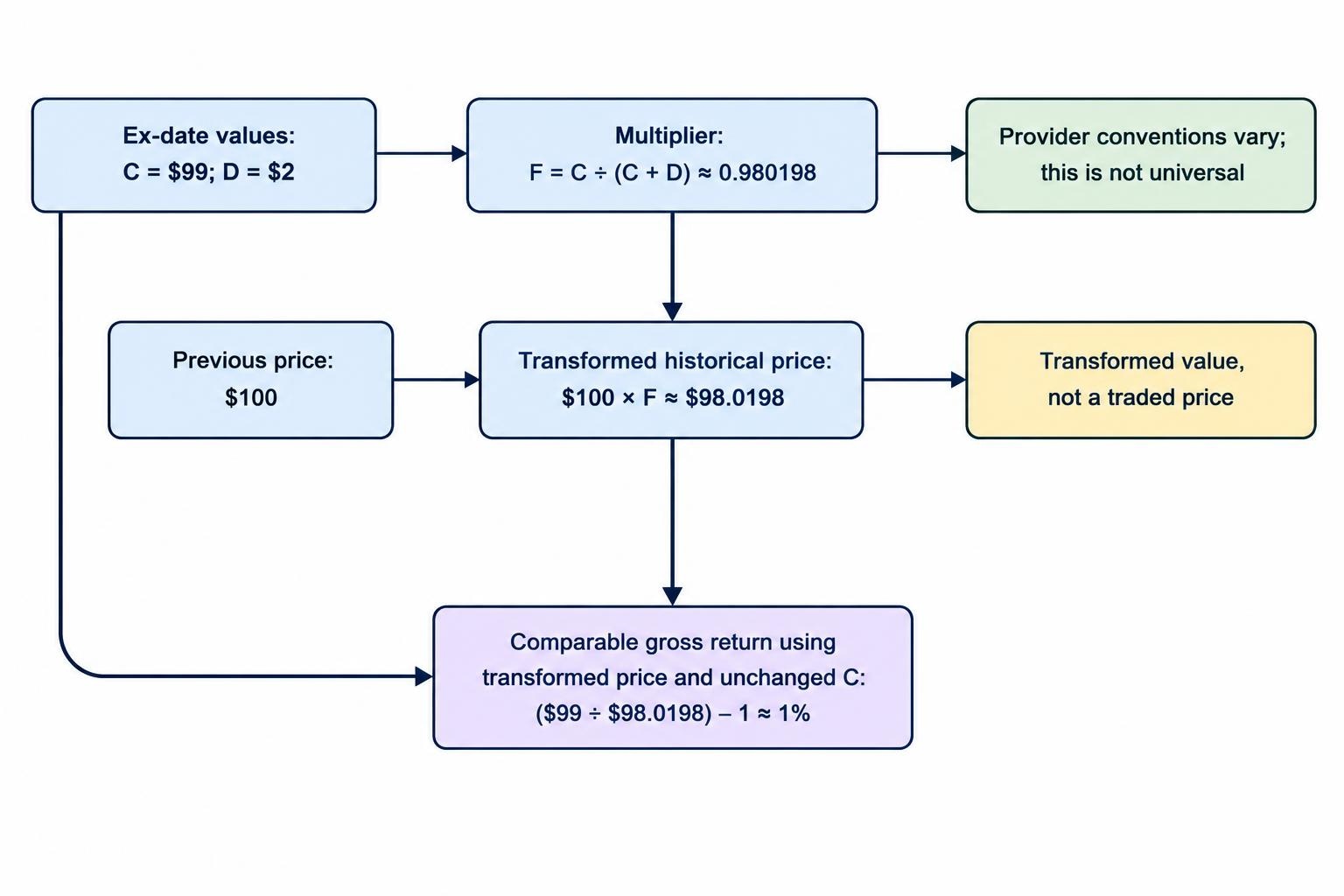
F = C ÷ (C + D)
Multiply earlier prices by F. Nasdaq Data Link documents the equivalent operation as dividing historical prices by (C + D) ÷ C in its Sharadar equity price adjustment documentation.
A Dividend Adjustment Example
Suppose a hypothetical stock closes at $100 before the ex-dividend date, distributes $2 per share, and closes at $99 on the ex-date. Assume no split, tax, or transaction cost.
The shareholder’s gross return is:
($99 + $2) ÷ $100 − 1 = 1%
Using the backward multiplier:
F = $99 ÷ ($99 + $2) = 0.980198…
The previous $100 close becomes approximately $98.0198. Comparing the unchanged ex-date close of $99 with $98.0198 produces the same 1% return.
This adjusted $98.0198 is not a price at which the stock traded. It is a transformed value used to calculate returns. That distinction matters when a backtest tries to turn an adjusted chart value into an executable order.
Do not assume every provider uses this formula. Record the provider’s convention, including the reference price and reinvestment timing, before comparing two adjusted histories. A label such as “adjusted close” is not a complete methodology.
Use the Correct Corporate Action Date
Keep the declaration date, ex-dividend date, record date, and payment date in separate fields. They answer different questions.
The ex-date governs the change in dividend entitlement for ordinary purchases: buying on or after that date generally does not entitle the buyer to the upcoming payment. The payment date identifies when the distribution is paid. The SEC’s explanation of dividend dates also covers exceptions for large distributions and stock dividends.
Use the confirmed event date rather than estimating it from a settlement rule. A correct formula applied to the wrong session still produces incorrect data.
In an account simulation, distinguish dividend entitlement from spendable cash. A model can recognize a dividend receivable when entitlement is established, then move it into cash on payment. A total return series that assumes earlier reinvestment answers a different question from a cash account that waits for payment.
Store the announcement timestamp too. An event’s effective date tells the adjustment engine when to change the share or return basis; the announcement timestamp tells a research system when the information became available.
Keep Open, High, Low, Close, and Volume Consistent
Adjusting only the closing price while leaving the open, high, and low untouched creates mixed units. That can corrupt range calculations, gap measurements, and stop simulations.
Check the actual fields returned by an endpoint. For example, Alpha Vantage’s daily adjusted endpoint documentation distinguishes raw daily open, high, low, close, and volume from its adjusted close field. An endpoint called “adjusted” does not necessarily return adjusted values in every column.
If the provider’s method applies one multiplicative factor to every price in a daily bar, derive the factor as:
Price factor = adjusted close ÷ corresponding raw close
Apply that factor to the raw open, high, and low to construct a bar on the same adjusted basis. First confirm that the two close fields share the same session and underlying price definition.
Maintain a separate split factor for volume. A cash dividend does not create additional shares, so do not adjust share volume using a combined split and dividend price factor.
For the hypothetical 2-for-1 split, a $120 price multiplied by 800,000 shares equals $96 million. Its adjusted equivalents, $60 multiplied by 1.6 million shares, give the same result. Dividend adjustment has no corresponding share-count conversion. Use raw prices and raw volume when estimating historical traded value.
Using Adjusted Data in a Backtest
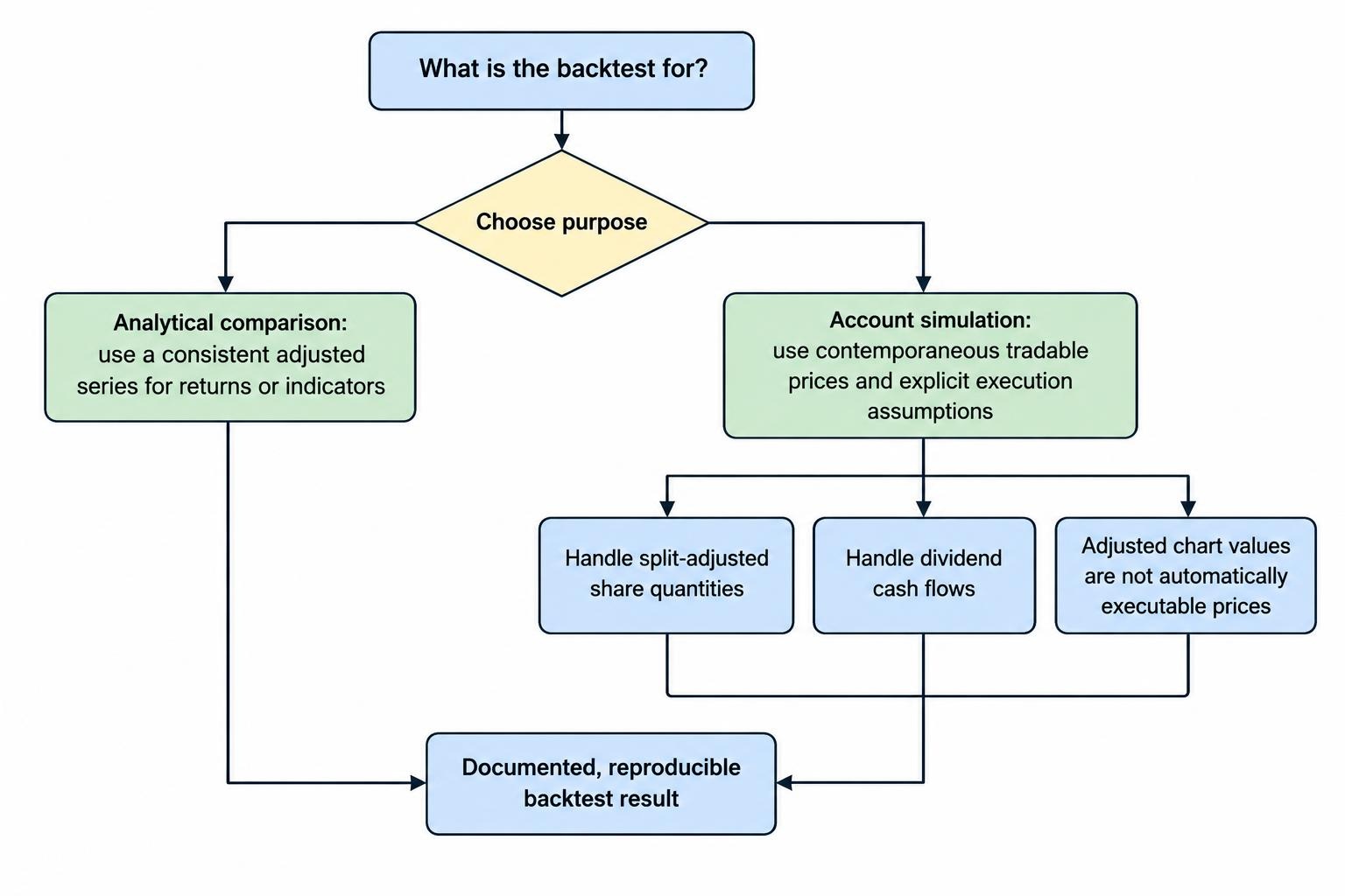
A practical design keeps analytical prices separate from execution prices. Use a consistent adjusted series where the strategy requires comparable prices or returns. Use historical tradable prices, share quantities, and explicit corporate action accounting to simulate the account.
This separation belongs in the rules for backtesting an automated trading strategy, not as an undocumented repair after the results look strange.
Do Not Count Dividends Twice
If portfolio performance is calculated from a return series that already incorporates dividends, adding those same dividends as extra profit overstates performance.
Choose an accounting approach and document it. A simplified fully invested return model can compound an appropriate total return series. A trade-by-trade account model can use raw execution prices, update holdings for splits, and track dividends separately. Switching between the two halfway through a calculation is where the trouble starts.
Adjust Positions as Well as Data
A split changes the share units of an open position. A hypothetical holding of 100 shares becomes 200 after a 2-for-1 split. Its equivalent per-share entry price halves.
The simulation also needs explicit treatment for working orders, fractional entitlements, and cash in lieu where relevant. Do not assume that adjusting the chart has adjusted the account. Price history and position accounting are separate records.
Watch Absolute Price Rules
Consider a strategy that buys only stocks trading above $10. If a later split changes a historical $40 observation into a latest-basis adjusted price of $8, applying the $10 threshold to that adjusted value changes the historical eligibility decision.
Use the contemporaneous price for a rule about the price actually quoted then. The same caution applies to fixed dollar stops, share-count constraints, and price-based eligibility filters.
Not every backward adjustment creates a false signal. Multiplying an entire lookback window by the same positive factor leaves percentage returns and a price-to-moving-average ratio unchanged. Test whether the rule depends on absolute units or relative relationships. The broader controls are covered in avoiding look-ahead bias and overfitting.
A Reliable Corporate Action Adjustment Workflow
Preserve raw data before creating adjusted versions. Store the corporate action ledger separately, with the security identifier, event type, ratio or cash amount, currency, relevant dates, and retrieval timestamp. Keep corrections rather than overwriting the evidence needed to reproduce an earlier run.
Next, choose an adjustment basis and write down its purpose. “Adjusted to the final session for chart comparison” is useful documentation. “Cleaned prices” is not.
Validate known events before processing the full universe. Test a forward split, a reverse split, an ordinary dividend, and multiple events. Check that split ratios run in the correct direction and that prices and share quantities use compatible units.
When a split and dividend share an effective date, confirm whether the dividend amount is quoted per old share or per new share. Normalize those units before combining the calculations. Do not assume the multiplication order will repair a mismatched cash amount.
Flag special dividends, spin-offs, rights distributions, and merger proceeds for event-aware handling rather than forcing everything through the ordinary dividend formula. Also flag missing prior closes and implausible adjustment factors for review.
Finally, save the data version, event ledger version, adjustment method, and base date with each research result. The objective is not the smoothest chart. It is a reproducible series that measures the intended return while keeping historical trading prices, share units, and cash flows straight.